Tutorial

ASAP CTX Walkthrough

Overview

There are multiple ways to use ASAP to produce DEMs. We will start with making a CTX DEM. The primary intended way to use asap is to use the notebook-based workflow commands through the command-line interface. These notebook-based workflow commands take a few parameters and will run a dozen or so individual steps serially. They are long-running commands for a single node, so using the nohup command is recommended to execute the program in the background. As the notebook workflow runs, various log files will appear in the directory and an output Jupyter notebook file containing all the logs when the program finishes. If the user is curious, a full_log.log file can be “tailed” by the user.

just run: asap ctx notebook_pipeline_make_dem

We assume the user has already activated their conda environment and are in a new empty directory. To start we need to select two CTX image IDs that we want to make a DEM of. All the steps to find and select CTX image IDs are outside of the scope of this tutorial for now. But in any case we will use a stereo pair of CTX data over Sera Crater in Arabia Terra, Mars.

Our image Ids are B03_010644_1889_XN_08N001W and P02_001902_1889_XI_08N001W. Let’s go ahead and take a look at them to see if there are any hazes or other issues.

B03_010644_1889_XN_08N001W

P02_001902_1889_XI_08N001W

They look great!

We will also need a stereo.default file, I will use one provided with the Ames Stereo Pipeline for a CTX image pair in their documentation: stereo.nomap. Selecting the correct parameters for a given pair is outside of the scope for this tutorial, but the Ames Stereo Docs are a good place to start to learn more about the various parameters.

Now that we have all of our components we are ready to run the ASAP notebook workflow:

nohup asap ctx notebook_pipeline_make_dem B03_010644_1889_XN_08N001W P02_001902_1889_XI_08N001W ./stereo.nonmap &

Again, we use the “nohup … &” to run our command in the background, on a 8 core machine this step can take half an hour or so. If you want to produce a DEM faster, you can choose lower resource parameters for ASP by editing the stereo.default file. Alternatively, you can also tell ASAP to make a lower-resolution DEM by specifying a downscale parameter, ie ‘–downscale 4’ to reduce the images by a factor of 4 in resolution. This one command will run several steps, replicating the workflow of the asp_scripts project. A notebook file, which default to be named “log_asap_notebook_pipeline_make_dem.ipynb” will also be created which we will explore later below.

Inspecting outputs

The notebook workflow produces a number of visualization products, some can be viewed using various ASP tools, some are produced by ASAP for viewing directly in the output notebook logs.

The Good Pixel Maps help quickly visualize if ASP is able to make sense of the provided images.

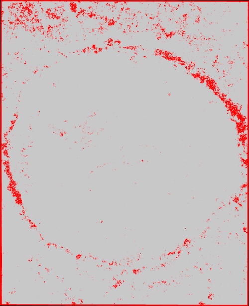
Good Pixel Map from first pass DEM from step 1.

Hillshaded products quickly convey the textural quality of the DEMs.

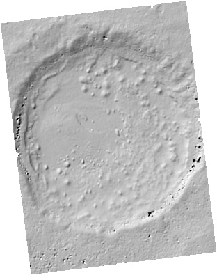
Hillshaded low-resolution DEM from step 1.

The final data products for CTX are located in the diretory: ID1_ID2/results_map_ba/dem_align/ where ID1 & ID2 are our CTX image ids. The final science-ready DEM file ends with the extension _DEM-adj.tif, the “adj” indicates the file is adjusted to the geoid. The final orthorectified images end with _DRG.tif. By default, for CTX images, ASAP will produce 6-meter orthorectified images and 24 meter DEMs. CTX data generally has better-than 6 meter GSD (~5.5 Meters per pixel), but the GSD is rounded up to produce conservative results for safety. This behavior can be overridden by the users at runtime using the ‘dem_gsd’ and ‘img_gsd’ command-line arguments. For more information regarding the various output files from Ames Stereo, please see their docs.

Congratulations, you have just made a DEM with ASAP!